Category: Tableau

Installing Tableau Server on Linux – Tableau 2021.1 Edition
It’s been over 2 years since we wrote our original blog post on installing Tableau Server on a Linux machine, to date it remains our most trafficked blog post. Since Tableau has continued to release new versions, we decided it was time to update our blog to reflect a new deployment.

Just like before, we’re starting with a fresh OS installation, still using Ubuntu LTS 16.04 (hey, it’s LTS for a reason!). We’ve upgraded our hardware, this time we’re installing on an actual data center server, an HP ProLiant ML350 Gen9 8-Port, with the following specs:
- (2) 2.6 GHz 8 Core Intel Xenon Processors with 20MB Cache (e5-2640v3)
- 128 GB Memory PC4-17000R (8 x 16GB sticks)
- 250 GB SSD
Tableau Server 2021.1 just released, so we’re installing the latest and greatest version. Since we’re on a Debian like distribution of Linux, we’ll use the .deb file type.

We still like following along to Everybody’s Install Guide that Tableau makes available. This is great for an IT generalist or someone doing a POC installation of Tableau Server. It gives you start to finish the steps you need to take and links out to many important knowledge articles along the way.

Before you get started, make sure the user you’ll be doing the installation with on the Linux machine can sudo – meaning it can perform operations like root. This will be necessary throughout the course of the installation. You’ll also want to do a general update on the OS.
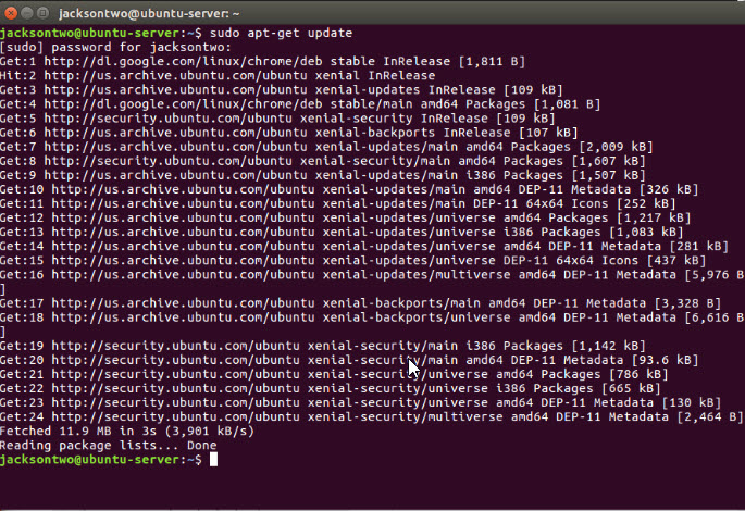
```
sudo apt-get update
```
If you’re following along with the guide mentioned above, Step 1 of the deployment is to install the Tableau Server package and start Tableau Services Manager (TSM). Since we’ve got a version of Linux with a GUI, we did this by downloading from the webpage. If instead you are downloading onto a headless server, you’ll want to install curl and use it to download the installer. Alternatively you can use wget.
```
sudo apt install curl
curl -O https://downloads.tableau.com/esdalt/2021.1.0/tableau-server-2021-1-0_amd64.deb
```
```
sudo apt-get install wget
wget https://downloads.tableau.com/esdalt/2021.1.0/tableau-server-2021-1-0_amd64.deb
```
Depending on where you are within the terminal, you may want to navigate to a different folder before downloading the file. After you download the installer, but before you execute it, you’ll want to make sure you’ve got gdebi-core installed.

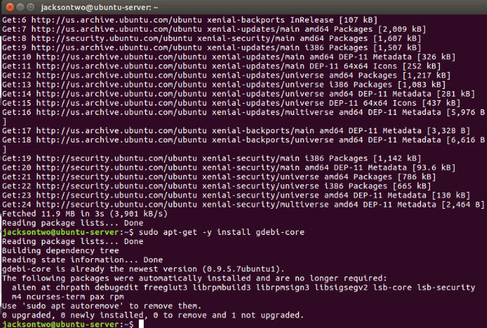
Now we’re all set and ready to actually install Tableau Server! In your terminal navigate to the folder where the file was saved.
```
cd Downloads
sudo gdebi -n tableau-server-2021-1-0_amd64.deb
```
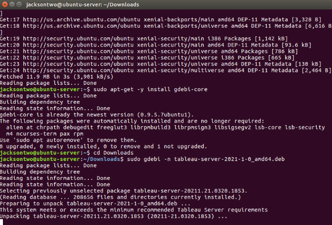
From here, you’ll open the package and unpack Tableau Server. Tableau does you a solid and will provide the exact location and command to run the installation script. Don’t forget that tab-complete is your friend in the terminal.
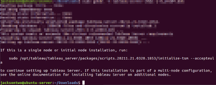
```
sudo /opt/tableau/tableau_server/packages/scripts.20211.21.0320.1853/initialize-tsm --acceptaeula
```
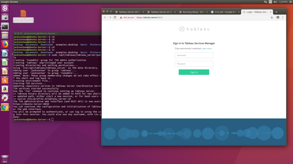
Tableau will now begin the initial installation. This happens in 2 steps, first it will go through a short process to initialize, then you’ll be prompted to continue the install either via the TSM GUI (servername:8850) or via TSM command line. It even reminds you what your initial user credentials should be for the next step (which are typically the same as the user you’re logged in as) and what the default URL for the server is.

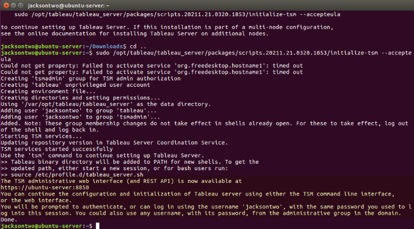
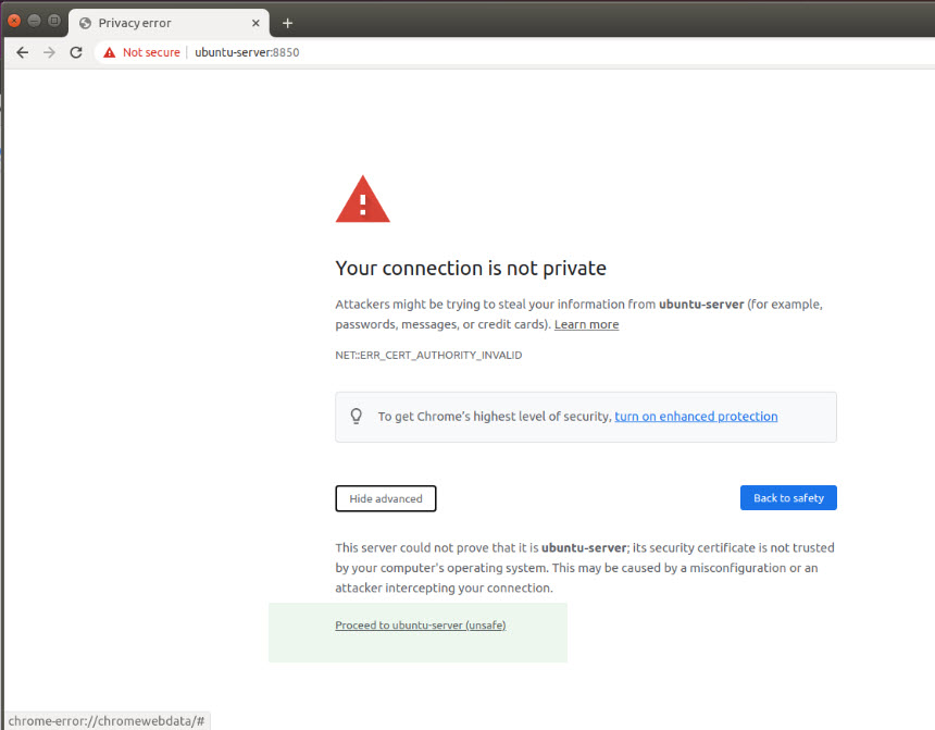
If you’re working in the TSM GUI (from browser), now is the time to go to the TSM page. Tableau Server generates a self-signed SSL certificate when it initializes, so you may see an untrusted message in your browser. You can go ahead and bypass this error message to login to TSM.

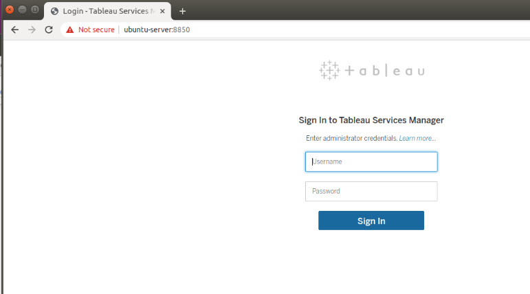
Remember, your user name and password used to log in to the machine are what you’ll enter here. The time to enter users will come after you decide which Identity Store method you’ll be using.

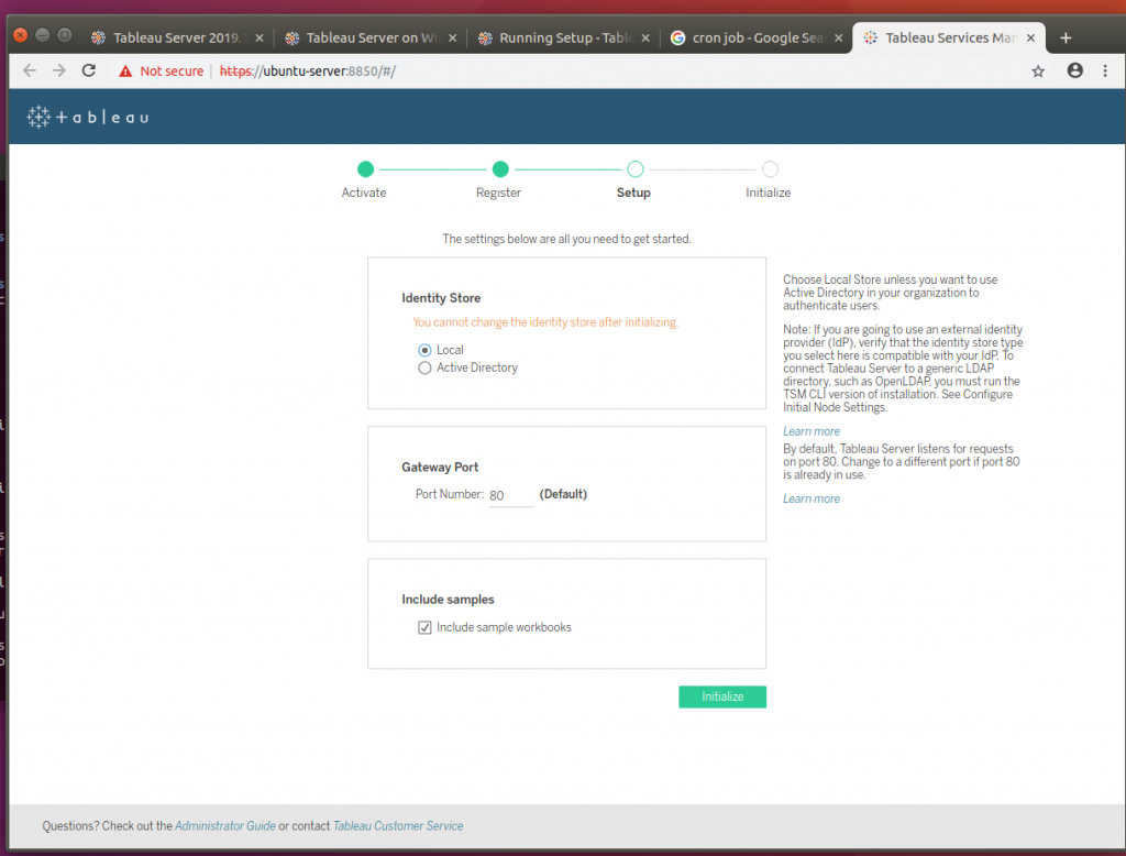
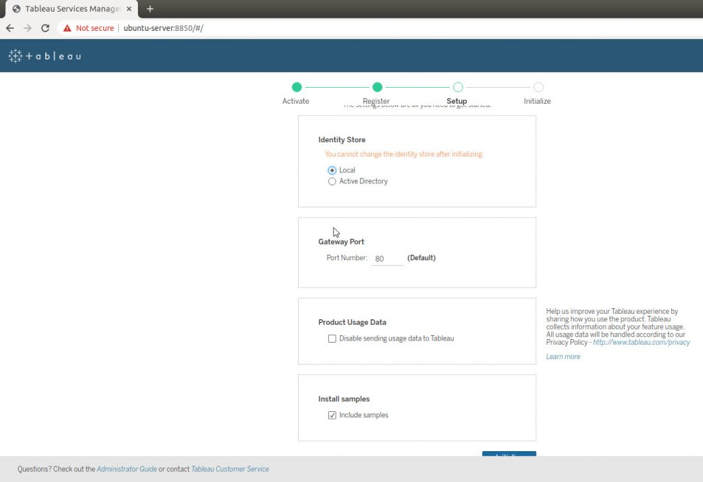
You’ll be prompted to register the product, and then get hit with 4 immediate configuration requests. Identity Store is the most serious setting on this page, because once you set it, you can’t change it. For our deployment we’ll be using Local (meaning we’ll create user names and the Server will manage passwords) authentication. If instead you wanted to do Active Directory (or another LDAP), selecting that option will prompt you to fill in the name of the AD domain.

If you’re unsure of any of these initial settings, remember you can hover over the section to get a nice paragraph from Tableau about the setting’s purpose. They also have a link at the bottom for the Administrator’s Guide.

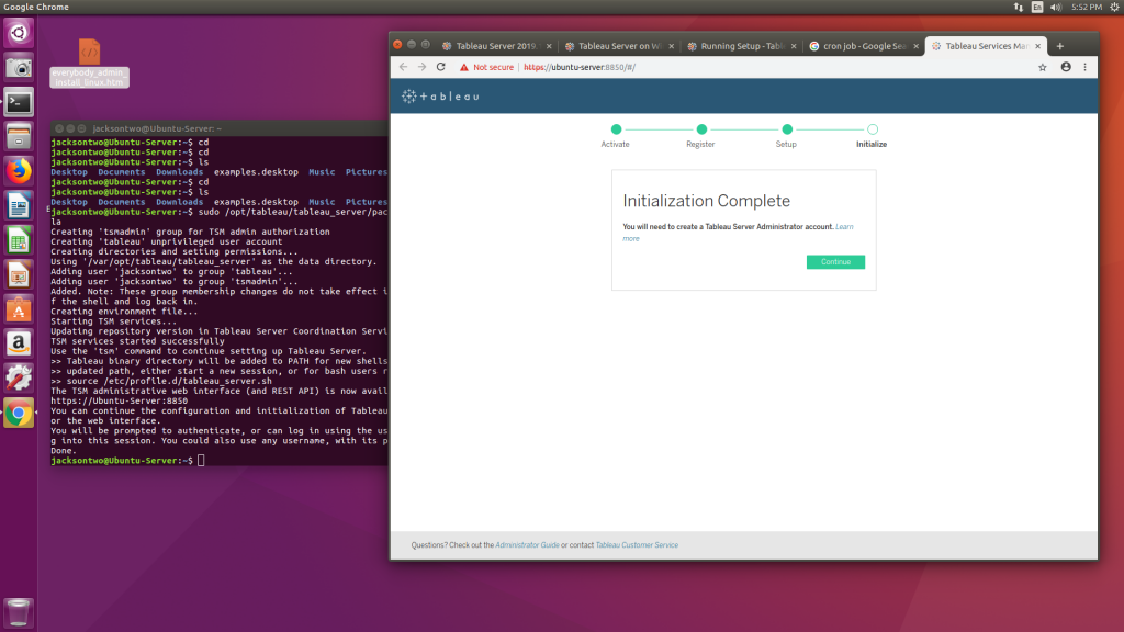
For this next part, go ahead and make yourself a cup of coffee, because this is the longest part of the install. Tableau will go through initializing several components, including setting the initial topology. Depending on the hardware you’re running, this can take anywhere from 10 to 30 minutes.

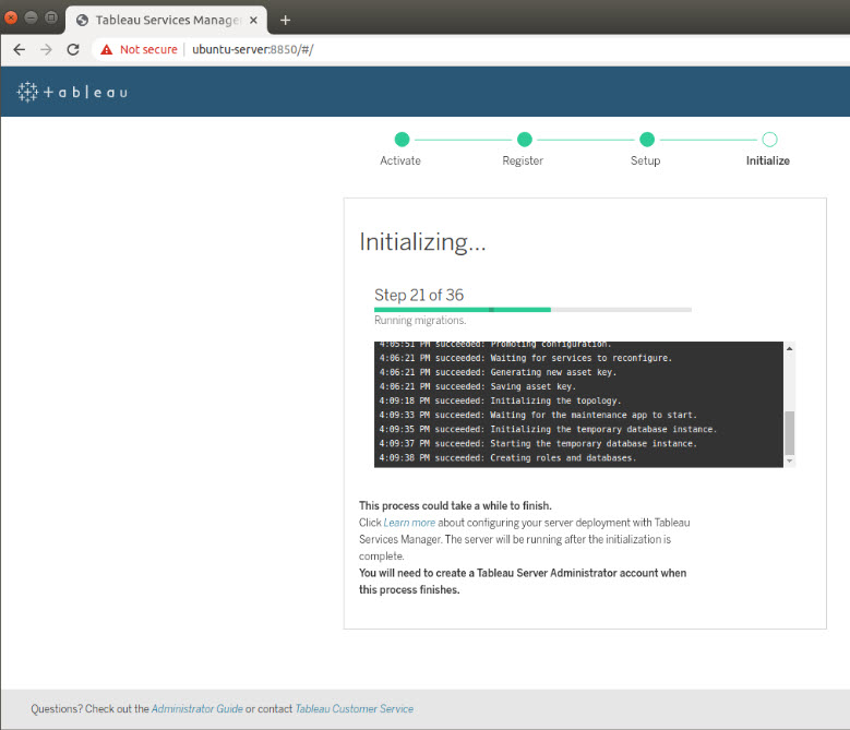
Once this step completes your Server is nearly up and running. The webpage should prompt you to create your first Administrator account. If you’re using Local Directory, you can use any username you’d like (for simplicity we’re repeating the same username). If you’re using Active Directory, you’ll have to pick a user ID associated with the domain. The password for AD will be slightly different, instead of requesting you to generate one, you’ll simply be prompted to enter your password.

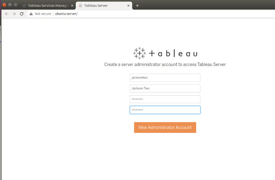
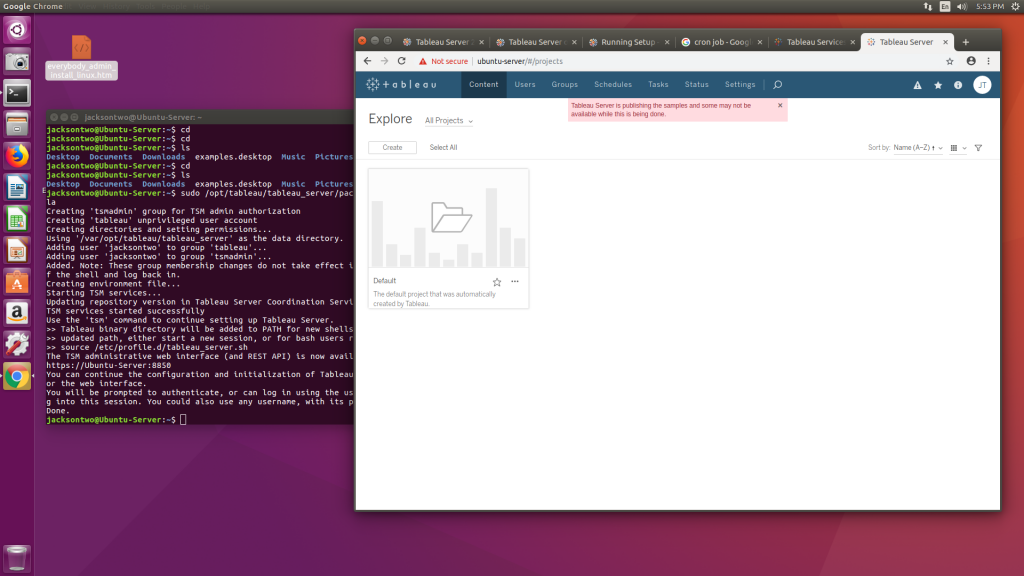
Once you create an administrator account, you’ll be immediately logged into the Server environment (in fact you can see in the screenshot above, it opens a new tab for the server and keeps TSM up).

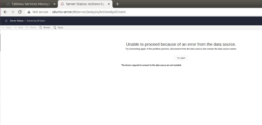
Now, because it’s a Linux installation, as a final step you’ll want to download and install the drivers for PostgreSQL. Remember that Tableau Server uses PostgreSQL as the backend to store all of your content, so you’ll need to install the driver to see the Administrator views (located in Server Status).

New with 2020.4 +, is a new version of the PostgreSQL database. In these newer installations, you’ll have to add a JDBC (previously we would use an ODBC) driver to connect to PostgreSQL. So make sure you navigate over to the Drivers Download page Tableau provides. At time of writing, Tableau linked to the following driver: https://downloads.tableau.c om/drivers/linux/postgresql/postgresql-42.2.14.jar. If you’ve got a GUI you can use, go ahead and download it from the page – otherwise use curl or wget to download the .jar.
```
curl -O https://downloads.tableau.com/drivers/linux/postgresql/postgresql-42.2.14.jar
wget https://downloads.tableau.com/drivers/linux/postgresql/postgresql-42.2.14.jar
```
Final steps are to create and drop the driver into /opt/tableau/tableau_driver/jdbc, which Tableau mentions you may have to manually create. We did have to create it, so here’s the code snippet. Make sure you’re at the root when you try to navigate to /opt/tableau. This is also a protected folder, so you’ll need to sudo to create the new directories.
```
cd /opt/tableau
sudo mkdir tableau_driver
cd tableau_driver
sudo mkdir jdbc
```
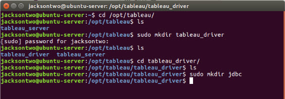
And finally, copy the file into the new directory you just created.
```
sudo cp postgresqul-42.2.14.jar /opt/tableau/tableau_driver/jdbc
```
After we dropped the JDBC driver, our Server install still wasn’t loading the visualizations for the Admin views. So we went ahead and restarted the Tableau Server. That immediately cleared up the issue and we could see our admin views!

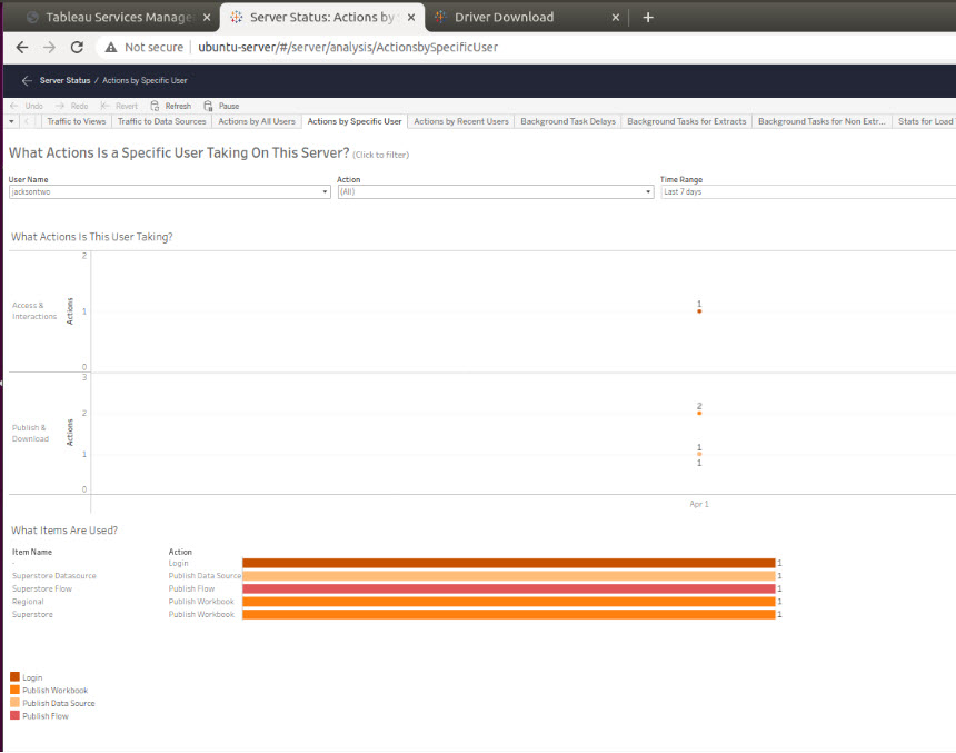
And that’s it – installation is complete! There are definitely more customizations and configurations we’re sure you’ll want to implement, but pause for a moment and rejoice in setting up a platform for people to interact with their data.
April 1, 2021
Installing Tableau Server on Linux (Ubuntu LTS 16.04)
Over the past six months we’ve noticed a trend – most of our clients are interested in installing Tableau Server on Linux (opposed to Windows). In fact at the recent Tableau Conference, over 25% of new Server installs were attributed to Linux distributions.

With that sense of growing popularity, we wanted to take some time and walk through a basic installation on Linux. This is similar to our previous post deploying Tableau Server on Azure and is not meant to be a template for sophisticated installations. Instead you can consider this a primer of what you can expect when installing on a Linux machine.

To start the process you’ll need a fresh copy of Linux on a machine that meets Tableau Server’s minimum hardware requirements (64-bit 2 core processor, 8 GB RAM, 15 GB free space). We chose to install Ubuntu LTS 16.04 via flash memory onto a system with 16 GB RAM, 500 GB SSD, and an Intel i7 4770 3.4 GHz quad-core processor. The server was re-purposed from a previous life as a mid-weight gaming PC.

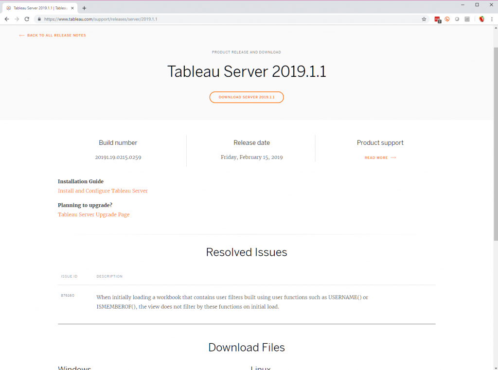
At time of writing we downloaded Tableau Server 2019.1.1, selecting the .deb options which aligns with the operating system we selected.

Throughout the process we like to reference the Everybody’s Install guide that Tableau provides. It helps ensure we don’t forget any steps and use the major content chapters as guides on the outline of the entire process.

Following along with Step 1: Install Tableau Server package, we quickly went through the process of updating applications on the system.
```
sudo apt-get update
```
The installation process then directs you to install gdebi, which allows installation of deb packages (the file type that the Tableau Server install package is).
```
sudo apt-get -y install gdebi-core
```
Finally it’s time for the good stuff – actually installing the software itself onto the server. To do this you’ll run the last command, with the expectation that you’ll know to navigate to the directory where the file is located. For our installation the location is Downloads.
```
cd Downloads
sudo gdebi -n tableau-server-2019-1-1_amd64.deb
```
This is a relatively quick process and gives you a good ending snippet of code for next steps – to run the initialization script and accept the EULA. They’ve provided the full path of the script, so it’s best to start at the root when executing.
```
sudo /opt/tableau/tableau_server/packages/scripts.2019.1.19.0215.0259/initialize-tsm --accepteula
```
And as the last 2 lines indicate, you’re now prompted to login to Tableau Services Manager (TSM) for the first time using your administrator credentials (which are most likely the username and password you’re already logged into).

There’s then a 4 step process to register your Tableau Server and do some initial configuration. The first option you’ll be hit with is Identity Store. I don’t remember this in the past, but there’s now a handy mouse-over detail to the right of the option box to help guide you on what to select. We chose Local – meaning we won’t be relying on Active Directory for user authentication.

Tableau Server then runs through it’s final initialization process, displaying in a small window what it’s doing along the way. For reference, this took about 10 minutes to complete.

You’ll then be prompted to set up a Tableau Server Administrator account. This isn’t necessarily the same username and password as the machine the Server is on, rather it’s the user name of the person who will be managing the Tableau Server itself.

At this point you’ll jump directly into a fresh copy of Tableau Server, where it even includes an alert to let you know that the samples are still being generated.

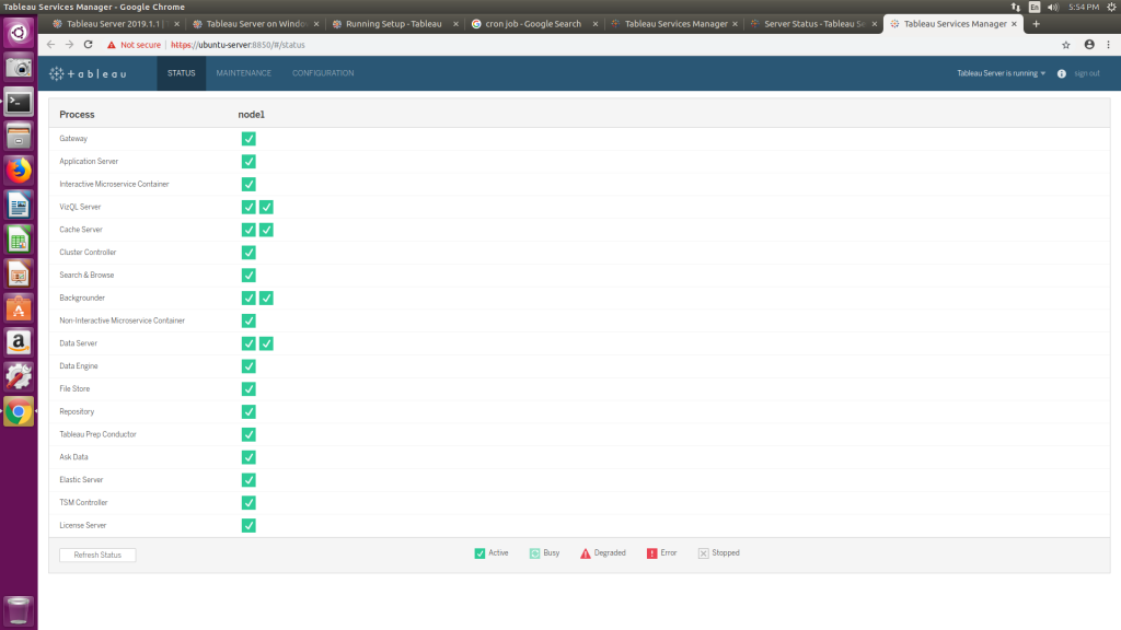
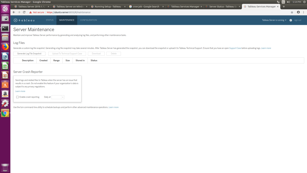
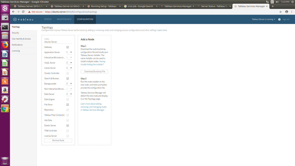
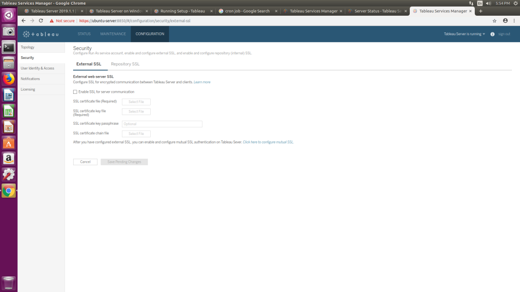
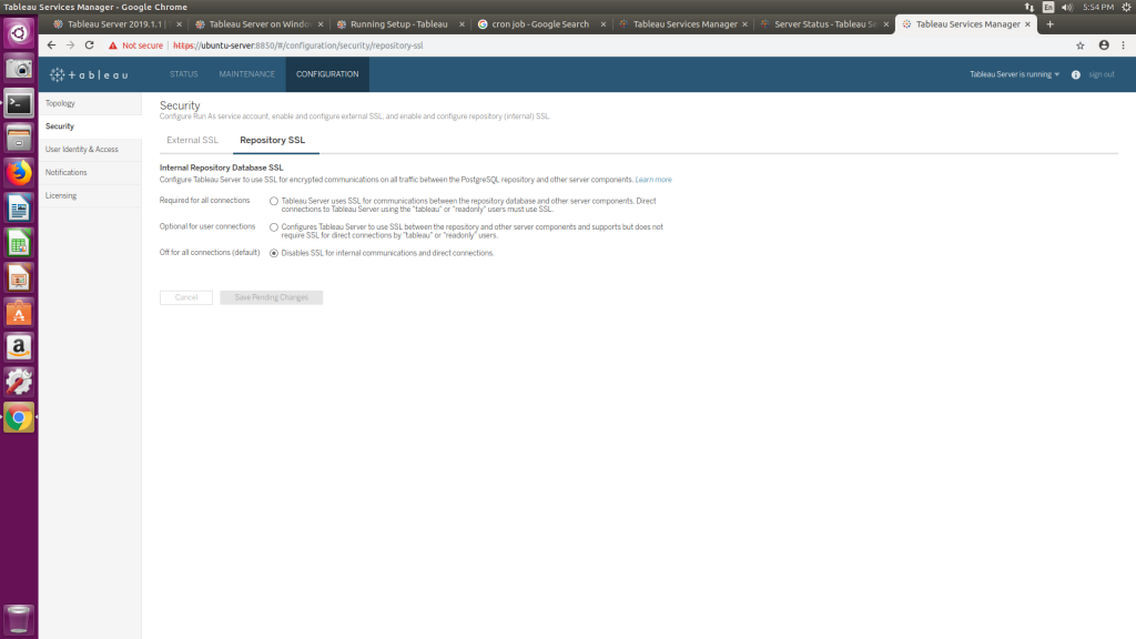
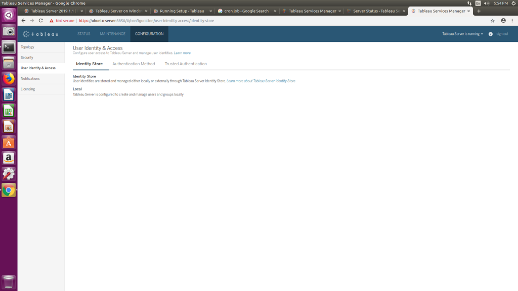
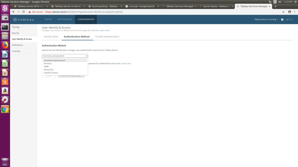
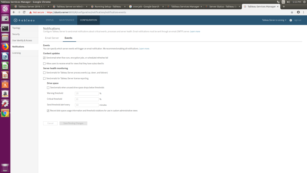
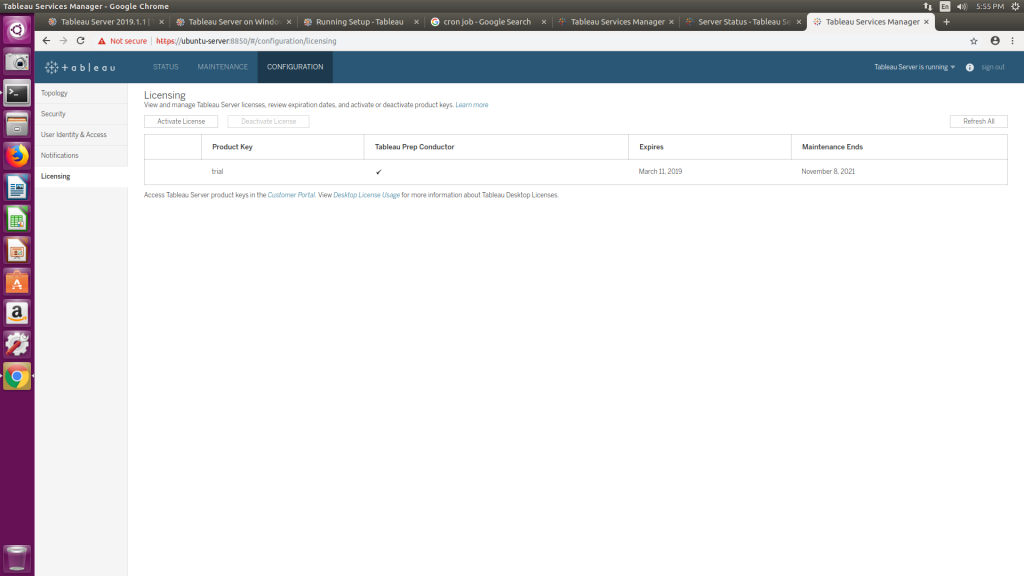
With the Server finally installed we like to go exploring in TSM (Tableau Services Manager). This is the front-end GUI that Server Administrators can access to do a variety of tasks, including restarting the server, adding licenses, generating logs, enabling SSL, and email/SMTP configuration.

We struggled in the past to find a picture of every screen within TSM, so we decided to include a gallery of each screen below. Click on each picture to see a full size version.
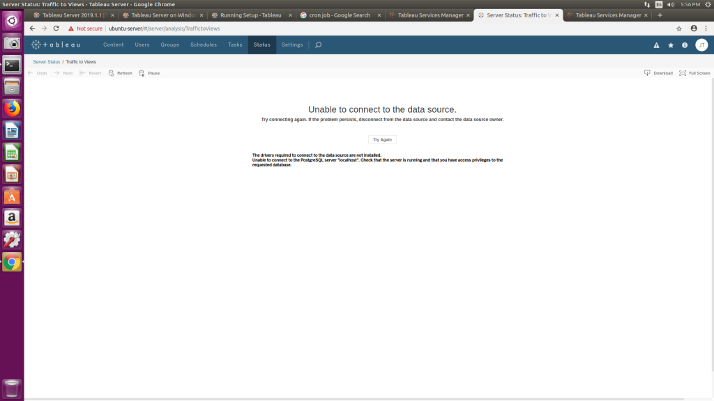
The last required step to getting started (at least from our perspective) is ensuring the administrator views work. This requires downloading an additional PostgreSQL driver for Linux (it is not bundled in the install). You’ll see this if the driver isn’t downloaded or isn’t installed properly.

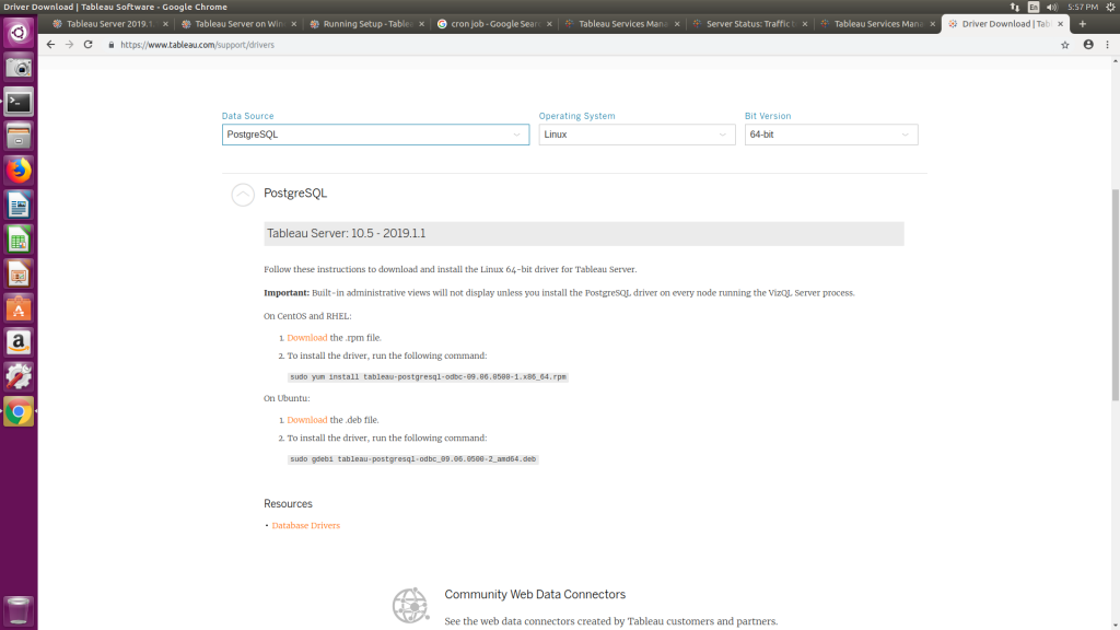
Our initial path forward was to go to Tableau Driver Downloads and download the appropriate driver (as listed).

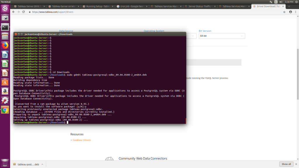
After downloading you’ll be able to run the command they provide in the terminal to install the driver. Remember to navigate to the directory the file is in (Downloads) first.
```
sudo gdebi tableau-postgresql-odbc_09.06.0500-2_amd64.deb
```
Worth mentioning, after we installed this driver the Administrator views were still not visible. And from our perspective it seems that there was an issue with the driver itself. So we chose to downgrade to an older version (that we knew worked from a previous install). We were able to locate driver version 9.5.3 via AWS.
```
https://s3-us-west-2.amazonaws.com/tableau-quickstart/tableau-postgresql-odbc_9.5.3_amdb64.deb
```
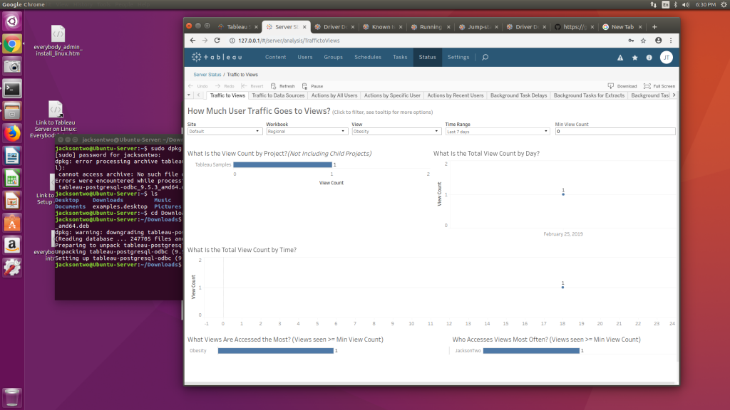
And after installing we finally got a look at those admin views!

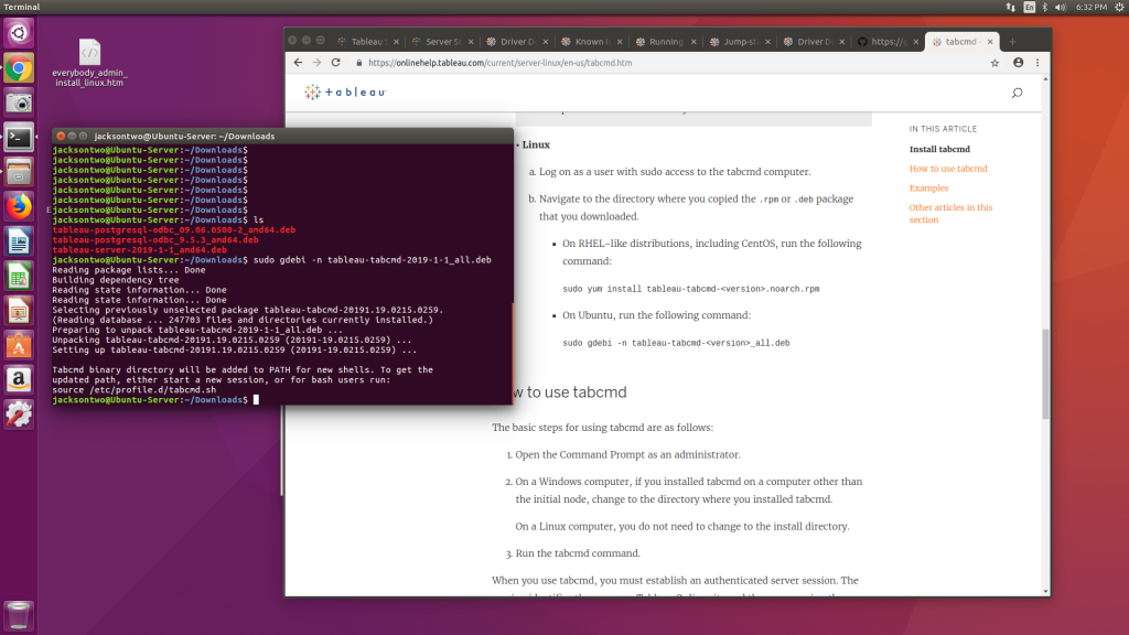
Two more steps we wanted to try out after installing. The first was installing tabcmd and making sure we could connect to the server. By now you’re a pro at navigating to the folder where the install is (and you know to pick the .deb file) – so getting to this step should be pretty easy.

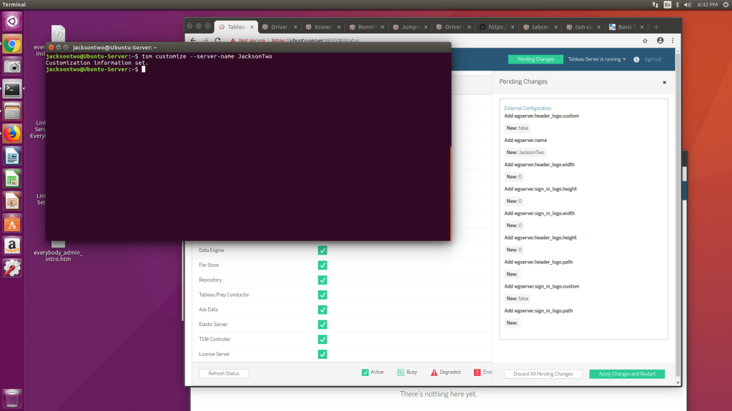
And our last step was to ensure the tsm command line client was working and to try out a command only available at this level vs. the TSM GUI. We chose to rename our server to JacksonTwo.

After renaming you’ll notice that we then navigated to the GUI TSM to see the pending changes that needed to be applied. The server required a restart for the name change to be applied. The final result is below, which was also taken on a Windows machine on our network.

And with that, a fresh install of Tableau Server on Linux has been installed and quickly customized. Keep a close eye on the blog – over the coming posts we’ll be continuing to dive deeper into Tableau Server.
February 25, 2019
Dynamic Quantile Map Coloring in Tableau Desktop
Last week at Tableau’s customer conference (TC18) in New Orleans I had the pleasure of speaking in three different sessions, all extremely hands on in Tableau Desktop. Two of the sessions were focused exclusively on tips and tricks (to make you smarter and faster), so I wanted to take the time to slow down and share with you the how of my favorite mapping tip. And that tip just so happens to be: how to create dynamic coloring based on quantiles for maps.

First, a refresher on what quantiles are. Quantiles are points that you can make within a data distribution to evenly cut it into equal intervals. The most popular of the quantiles is the quartile, which partitions out data into 0 to 25%, 25 to 50%, 50 to 75%, and 75 to 100%. We see quartiles all the time with boxplots and it’s something we’re quite comfortable with. The reason the quantile is valuable is that it lines up all the measurements from smallest to largest and buckets them into groups – so when you use something like color, it no longer represents the actual value of a measurement, but instead the bucket (quantile) that the measurement falls into. These are particularly useful when measurements are either widely dispersed or very tightly packed.

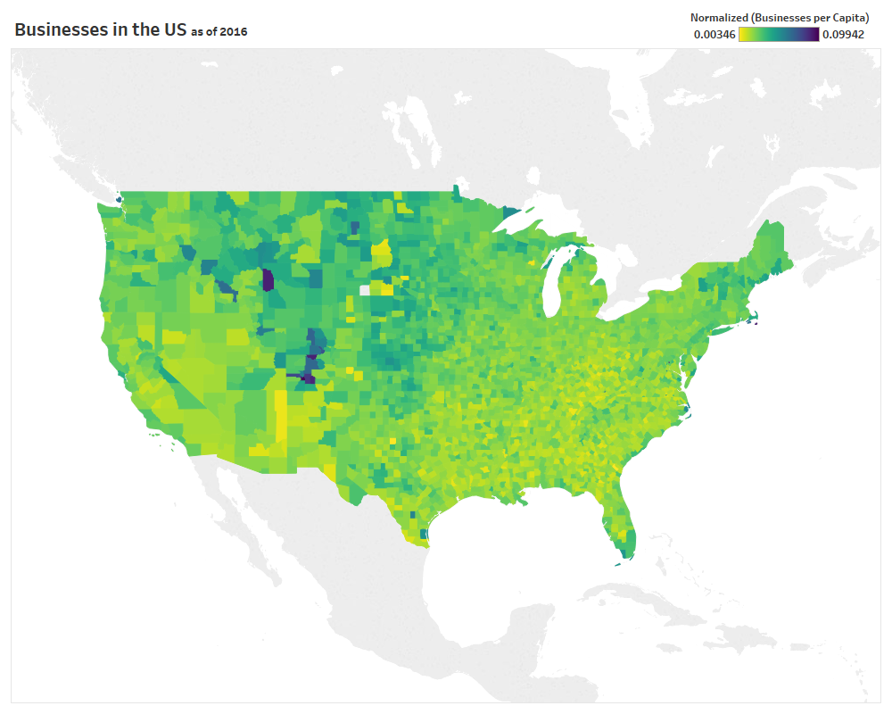
Here’s my starting point example – this is a map showing the number of businesses per US county circa 2016.

The range of number of businesses per county is quite large, going from 1 all the way to about 270k. And since there is such a wide variety in my data set, it’s hard to understand more nuanced trends or truly answer the question “which areas in the US have more businesses?”

A good first step would be to normalize by the population to create a per capita measurement. Here’s the updated visualization – notice that while it’s improved, now I’m running into a new issue – all my color is concentrated around the middle.

The trend or data story has changed, my eyes are now drawn toward the dark blue in Colorado and Wyoming, but I am still having a hard time drawing distinctions and giving direction on my question of “which areas in the US have the most businesses?”

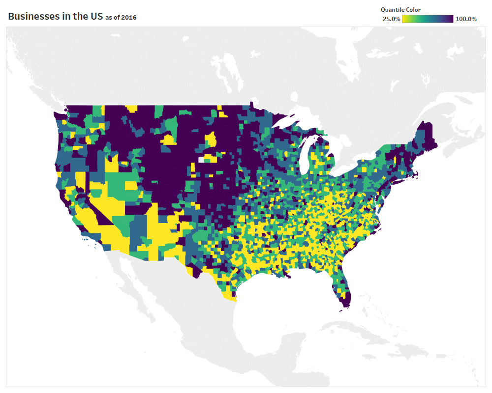
So as a final step I can adjust my measurements to percentiles and bucket them into quantiles. Here’s the same normalized data set now turned into quartiles.

I now have 4 distinct color buckets and a much richer data display to answer my question. Furthermore I can make the legend dynamic (leading back to the title of this blog post) by using a parameter. The process to make the quantiles dynamic involves 3 steps:
1. Turn your original metric (the normalized per capita in my example) into a percentile by creating a “Percentile” Quick Table Calculation. Save the percentile calculation for later use.
2. Determine what quantiles you will allow (I chose between 4 and 10). Create an integer parameter that matches your specification.

3. Create a calculated field that will bucket your data into the desired quantile based on the parameter.

You’ll notice that the Quantile Color calculation depends on the number of quantiles in your parameter and will need to be adjusted if you go above 10.

Now you have all the pieces in place to make your dynamic quantile color legend. Here’s a quick animation showing the progression from quartiles to deciles.

The next time you have data where you’re using color to represent a measure (particularly on a map) and you’re not finding much value in the visual, consider creating static or dynamic quantiles. You’ll be able to unearth hidden insights and help segment your data to make it easier to focus on the interesting parts.

And if you’re interested in downloading the workbook you can find it here on my Tableau Public.
October 31, 2018
Without Water an Iron Viz feeder

Jump directly to the viz

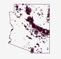
At the time of writing it is 100°F outside my window in Arizona and climbing. It’s also August and we’re right in the middle of feeder round 3 for Tableau Public’s Iron Viz contest. Appropriately timed, the theme for this round is water. So it’s only fitting that my submission for this round would take into consideration the mashup of these two and form my submission: Without Water, 2 decades of drought & damage in Arizona.

The Genesis of the Idea

I’ll start by saying that water is a very tricky topic. The commonplace of it makes searching for data and a narrative direction challenging. It’s necessary for sustaining life, so it seems to want to have a story tied directly to humankind – something closely related to water quality, water availability, loss of water – essentially something that impacts humans. And because it’s so vital, there are actually several organizations and resources doing fantastic things to demonstrate the points above. Unicef tracks drinking water and sanitation, Our World in Data has a lengthy section devoted to the topic, there’s the Flint Water Study, and the Deepwater Horizon oil spill.

This realization around the plethora of amazing resources associated with water led me to the conclusion that I would have to get personal and share a story not broadly known. So what could be more personal than the place I’ve called home for 14 years of my life: Arizona.

Arizona is a very interesting state, it’s home to the Grand Canyon, several mountain ranges, and of course a significant portion of the Sonoran desert. This means that in October it can be snowing in the mountains of Flagstaff and a stifling 90°F two hours south in Phoenix. And, despite the desert, it needs water. Particularly in the large uninhabited sections of the mountains covered with forests. Getting to the punchline: since my time in Arizona, the state has been in a long sustained drought. A drought that’s caused massive wildfires, extreme summer heat, and conversation thread that never steers far from the weather.

Getting Started

A quick google search led me to my first major resource: NOAA has a very easy to use data portal for climate data which includes: precipitation, various drought indices, and temperatures – all by month/state/and division. This served as the initial data set along with the joining of climate division shapefiles maintained by NCEI. Here’s the first chart I made showing the divisions by their drought index. This uses the long term Palmer Drought Severity Index and any positive values (non-drought) are zeroed out to focus attention on deficit.

My next major find was around wildfire data from the Federal Fire Occurrence website. Knowing that fire is closely associated with drought, it seemed a natural progression to include. Here’s an early iteration of total acres destroyed by year:

It’s clear that after 2002 a new normal was established. Every few years massive fires were taking place.

And after the combination of these two data sets – the story started developing further – it was a time bound story of the last 20 years.

Telling the Story

I headed down the path of breaking out the most relevant drought headlines by year with the idea of creating 20 micro visualizations. Several more data sources were added (including dust storms, heat related deaths, and water supply/demand). An early iteration had them in a 4 x 5 grid:

As the elements started to come together, it was time to share and seek feedback. Luke Stanke was the first to see and gave me the idea of changing from a static grid to a scrolling mobile story. And that’s where things began to lock into place. Several iterations later and with input from previous Iron Viz winner Curtis Harris – the collection of visualizations was starting to become more precisely tuned to the story. White space became more defined and charts were sharpened.

My final pass of feedback included outsourcing to Arizona friends (including Josh Jackson) to ask if it evoked the story we’re all experiencing and it’s what led to the ultimate change in titles from years to pseudo-headlines.

Wrapping Up

My one last lingering question: Mobile only or to include a desktop version? The ultimate choice and deciding factor was to create a medium and version that was optimized for getting to the largest end audience – thus, mobile only.

WITHOUT WATER

And now that all leads to the final product. A mobile only narrative data story highlighting the many facets of drought and it’s consequences for the state of Arizona. Click on the image to view the interactive version on Tableau Public.

click to view on Tableau Public

August 14, 2018
Building an Interactive Visual Resume using Tableau

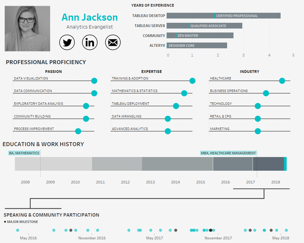
click to interact on Tableau Public

In the age of the connected professional world it’s important to distinguish and differentiate yourself. When it comes to the visual analytics space, a great way to do that is an interactive resume. Building out a resume in Tableau and posting it on Tableau Public allows prospective employers to get firsthand insight into your skills and style – it also provides an opportunity for you to share your professional experience in a public format.

Making an interactive resume in Tableau is relatively simple – what turns out to be more complex is how you decide to organize your design. With so many skills, achievements, and facts competing for attention, it’s important for you to decide what’s most important. How do you want your resume to be received?

In making my own resume, my focus was on my professional proficiency across larger analytics domains, strength in specific analytics skills, and experience in different in industries. I limited each of these components to my personal top 5, so that it is clear to the audience what areas hold the most interest for me (and I’m most skilled in).

Additionally, I also wanted to spend a significant amount of real estate highlighting my community participation. After plotting a gantt chart of my education and work experience, I realized that the last two years are jam packed with speaking engagements and activities that would be dwarfed on a traditional timeline. To compensate for this, I decided to explode the last two years into its own timeline in the bottom dot plot. This allowed for color encoding of significant milestones and additional detail on each event.

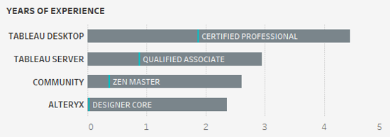
The other two components of the resume serve importance as well. I’ve chosen to demonstrate experience in terms of years (a traditional metric to demonstrate expertise) with the highest level of certification or professional attainment denoted along each bar. And finally, including a traditional timeline of my education and work experience. The “where” of my work experience is less important than the “what,” so significant detail was spent adding role responsibilities and accomplishments.

Once you’ve decided how you want to draw attention to your resume, it’s time to build out the right data structure to support it. To build out a gantt chart of different professional roles a simple table with the type of record, name of the role, start date, end date, company, flag for if it’s current role, and a few sentences of detail should suffice.

This table structure also works well for the years of experience and community involvement sections.

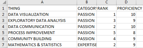
You may also want to make a separate table for the different skills or proficiencies that you want to highlight. I chose to make a rigid structured table with dimensions for the rank of each result, ensuring I wouldn’t have to sort the data over each category (passion, expertise, industry) once I was in Tableau.

Here’s the table:

That’s it for data structure, leaving style (including chart choices) as the last piece of the puzzle. Remember, this is going to be a representation of you in the digital domain, how do you want to be portrayed? I am known for my clean, minimalist style, so I chose to keep the design in this voice. Typical to my style, I purposely bubble up the most important information and display it in a visual format with supporting detail (often text) in the tooltip. Each word and label is chosen with great care. It’s not by mistake that the audience is seeing the name of my education (and not the institution) and the labels of each proficiency. In a world where impressions must happen instantaneously, it’s critical to know what things should have a lasting impact.

I also chose colors in a very specific manner, the bright teal is my default highlight color, drawing the eyes in to certain areas. However, I’ve also chosen to use a much darker gray (near black) as an opposite highlight in the bottom section. My goal with the dark “major milestones” is to entice the audience to interact and find out what major means.

The final product from my perspective represents a polished, intentional design, where the data-ink ratio has been maximized and the heart of my professional ambitions and goals are most prominent.

Now that you’ve got the tools – go forth and build a resume. I’m curious to know what choices you will make to focus attention and how you’ll present yourself from a styling perspective. Will it be colorful and less serious, will you focus on your employment history or skills? Much like other visualizations whatever choices you make, ensure they are intentional.

June 11, 2018
Blending Visualizations of Different Sizes
One of my favorite visualizations is the sparkline – I always appreciated how they are described by Edward Tufte “data-intense, design-simple, word-sized graphics.” Meaning the chart gets right to the point: conveying a high amount of information without sacrificing real estate. I’ve found this approach works really well when trying to convey different levels of information (detail and summary) or perhaps different metrics around a common topic.

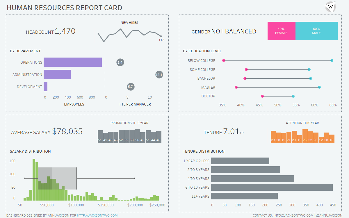
I recently built out a Report Card for Human Resources that aims to do just that. Use a cohort of visualizations to communicate an overall subject area and then repeat the concept to combine 4 subject/metric areas. Take a look at the final dashboard below.

click to view on Tableau Public

The dashboard covers one broad topic – Human Resources. Within it there are 4 sub-topics: number of employees, key demographics, salary information, and tenure. As your eyes scan through the dashboard, they likely stopped at the large call outs in each box. You’ve got your at-a-glance metrics that start to bring awareness to the topic.

But the magic of this dashboard lies in the collection of charts surrounding the call outs. Context has been added to surround each metric. Let’s go through each quadrant and unpack the business questions we may have.
1. How many active employees do we have?
2. How many new employees have we been hiring?
3. How many employees are in each department?
4. What’s the employee to leadership ratio?
The first visualization (1) is likely the one a member of management would want. It’s the soundbite and tidbit of information they’re looking for. But once that question is asked and answered, the rest of the charts become important to knowing the health of that number. If it’s a growing company, the conversation could unfold into detail found in chart 2 – “okay we’re at 1500 employees, what’s our hiring trend?” The same concept could be repeated for the other charts – with chart 4 being useful for where there might be opportunity for restructuring, adding management, or checking up on employee satisfaction.

The next quadrant focuses specificly on employee demographics. And the inclusion of it after employee count is intentional. It’s more contextual information building from the initial headcount number.
1. Do we have gender equity?
2. What is the gender distribution?
3. How does the inclusion of education level affect our gender distribution?
Again, we’re getting the first question answered quickly (1) – do we have gender equity? Nope – we don’t. So just how far off are we, that’s answered just to the right (2). The second chart is still a bit summarized, we can see the percentages for each gender, but it’s so rolled up that we’d be pressed to figure out how or where the opportunity for improvement might be. This is where the final chart (3) helps to fill in gaps. With this particular organization, there could be knowledge that there’s gender disparity based on levels of education. We don’t get the answers to all the questions we have, but we are starting to narrow down focus immensely. We could go investigate a potentially obvious conclusion and try to substantiate it (this company hires more men without any college experience).

The next quadrant introduces salary – a topic everyone cares about.
1. What’s the average salary of one of our employees?
2. Are we promoting our employees? (A potential influence to #1)
3. What’s the true distribution of salaries within our organization?
The design pattern is obvious at this point – convey most important single number quickly, and then dive into context, drivers, and supporting detail. I personally like the inclusion of the histogram with a boxplot, a simple way to apply statistics to an easily skewed metric. Even in comparing the average number to the visual median, we can see that there are some top heavy salaries contributing to the number. And what’s even more interesting about the inclusion of the histogram is the frequency of salaries around the $25k mark. I would take away from this section the knowledge of $78k, but also the visual spread of how we arrive at that number. The inclusion of (2) here serves mostly for a form of context. Here it could be that the organization has an initiative to promote internally and thus goes hand-in-hand with salary changes.

And finally our last section – focused closely on retention.
1. What’s our average employee tenure?
2. How much attrition/turnover do we have monthly?
3. How much seniority is there in our staff?
After this final quadrant, we’ve got a snapshot of what a typical employee looks like at this organization. We know their likely salary, how long they’ve been with the company, some ideas on where they’re staffed, and a guess at gender. We can also start to fill in some gaps around employee satisfaction – seems like there was some high turnover during the summer months.

And let’s not forget – this dashboard can come more to life by the inclusion of a few action filters. We’ve put down the groundwork of how we want to measure the health of our team, now it’s time to use these to drive deeper and more meaningful questions and analysis.

I hope this helps to demonstrate how the inclusion of visualizations of varying sizes can be combined to tell a very rich and contextual data story – perfect for understanding a large subject area with contextual indicators and answers to trailing questions included.
May 11, 2018
The Shape of Shakespeare’s Sonnets | #IronViz Books & Literature
Jump directly to the viz

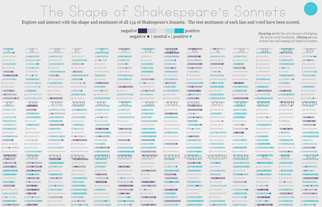
If it’s springtime that can only mean that it’s time to begin the feeder rounds for Tableau’s Iron Viz contest. The kick-off global theme for the first feeder is books & literature, a massive topic with lots of room for interpretation. So without further delay, I’m excited to share my submission: The Shape of Shakespeare’s Sonnets.

The genesis of the idea

The idea came after a rocky start and abandoned initial idea. My initial idea was to approach the topic with a meta-analysis or focus on the overall topic (‘books’) and to avoid focusing on a single book. I found a wonderful list of NYT non-fiction best sellers lists, but was uninspired after spending a significant amount of time consuming and prepping the data. So I switched mid-stream and decided to keep the parameters of a meta-analysis, but change to a body of literature that a meta-analysis could be performed on. I landed on Shakespeare’s Sonnets for several reasons:
- Rigid structure – great for identifying patterns
- 154 divides evenly for small multiples (11×14 grid)
- Concepts of rhyme and sentiment could easily be analyzed
- More passionate subject: themes of love, death, wanting, beauty, time
- Open source text, should be easy to find
- Focus on my strengths: data density, abstract design, minimalism
Getting Started

I wasn’t disappointed with my google search, it took me about 5 minutes to locate a fantastic CSV containing all of the Sonnets (and more) in a nice relational format. There were some criteria necessary for the data set to be usable – namely each line of the sonnet needed to be a record. After that point, I knew I could explode and reshape the data as necessary to get to a final analysis.

Prepping & Analyzing the Data

The strong structuring of the sonnets meant that counting things like number of characters and number of words would yield interesting results. And that was the first data preparation moment. Using Alteryx I expanded out line into columns for individual words. Those were then transposed back into rows and affixed to the original data set. Why? This would allow for quick character counting in Tableau, repeated dimensions (like line, sonnet number), and dimensions for the word number in each line.

I also extracted out all the unique words, counted their frequency, and exported them to a CSV for sentiment analysis. Sentiment analysis is a way to score words/phrases/text to determine the intention/sentiment/attitude of the words. For the sake of this analysis, I chose to go with a negative/positive scoring system. Using Python and the nltk package, each word’s score was processed (with VADER). VADER is optimized for social media, but I found the results fit well with the words within the sonnets.

The same process was completed for each sonnet line to get a more aggregated/overall sentiment score. Again, Alteryx was the key to extracting the data in the format I needed to quickly run it through a quick Python script.

Here’s the entire Alteryx workflow for the project:

The major components
- Start with original data set (poem_lines.csv)
  - filter to Sonnets
  - Text to column for line rows
  - Isolate words, aggregate and export to new CSV (sonnetwords.csv)
  - Isolate lines, export to new CSV (sonnetlines)
  - Join swordscore to transformed data set
  - Join slinescore to transformed data set
  - Export as XLSX for Tableau consumption (sonnets2.xlsx)
Python snippet

make sure you download nltk leixcons after importing; thanks to Brit Cava for code inspiration

The Python code is heavily inspired by a blog post from Brit Cava in December 2016. Blog posts like hers are critically important, they help enable others within the community do deeper analysis and build new skills.

Bringing it all together

Part of my vision was the provoke patterns, have a highly dense data display, and use an 11×14 grid. My first iteration actually started with mini bar charts for number of characters in each word. The visual this produced was what ultimately led to the path of including word sentiment.

height = word length, bars are in word order

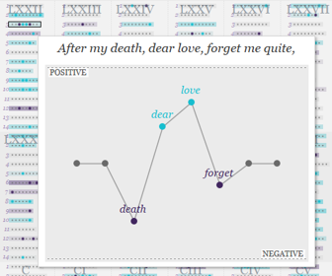
This eventually changed to circles, which led to the progression of adding a bar to represent the word count of each individual line. The size of the words at this point became somewhat of a disruption on the micro-scale, so sentiment was distilled down into 3 colors: negative, neutral, or positive. The sentiment of the entire line instead has a gradient spectrum (same color endpoints for negative/positive). Sentiment score for each word was reserved for a viz in tool tip – which provides inspiration for the name of the project.

Sonnet 72, line 2

Each component is easy to see and repeated in macro format at the bottom – it also gives the end user an easy way to read each Sonnet from start to finish.

designed to show the progression of abstraction

And there you have it – a grand scale visualization showing the sentiment behind all 154 of Shakespeare’s Sonnets. Spend some time reciting poetry, exploring the patterns, and finding the meaning behind this famous body of literature.

Closing words: thank you to Luke Stanke for being a constant source of motivation, feedback, and friendship. And to Josh Jackson for helping me battle through the creative process.

The Shape of Shakespeare’s Sonnets

click to interact at Tableau Public
May 8, 2018
Dying Out, Bee Colony Loss in US | #MakeoverMonday Week 18
Week 18 of Makeover Monday tackles the issue of the declining bee population in the United States. Data was provided by BeeInformed and the re-visualization is in conjunction with Viz for Social Good. Unfamiliar with a few of the terms – check out their websites to learn what Makeover Monday and Viz for Social Good are all about.

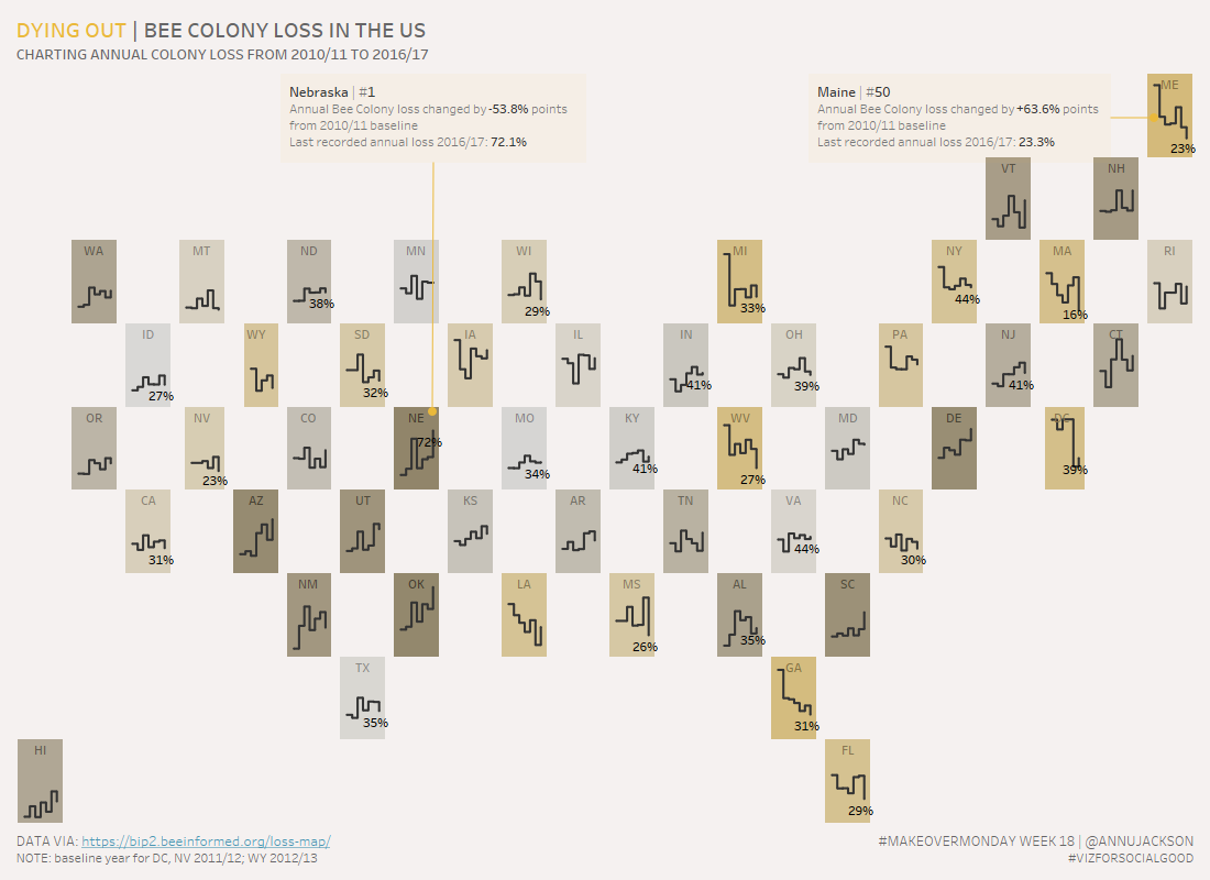
The original visualization is a filled map showing the annual percentage of bee colony loss for the United States. Each state (and DC) are filled with a gradient color from blue (low loss) to orange (high loss). The accompanying data set for the makeover included historical data back to 2010/11.

Original visualization | Bee Informed

Looking at the data my goal was to capitalize on some of the same concepts presented in the original visualization, but add more analytical value by including the dimension of time. The key component I was aiming to understand was that there’s annual colony loss, but how “bad” is the loss. The critical “compared to what” question.

My Requirements
- Keep the map theme – good way to demonstrate data
- Add in time dimension
- Keep color as an indicator of performance (good/bad indicator) – clarify how color was used
- Provide more context for audience
- Switch to tile map for skill building
- Key question: where are bees struggling to survive
- Secondary question: which states (if any) have improved
Building out the tile map and beginning to add the time series was pretty simple. I downloaded the hexmap template provided by Matt Chambers. I did a bit of tweaking to the file to change where Washington D.C. was located. Original file has it off to the side, I decided to place it in-line with the continental US to clean up the final look.

Well documented through the Tableau Community – the next step was to take the two data sources (bees + map) and blend them together. Part of that process includes setting up the relationship between the two data sources and then adding them both to a single view:

setting up the relationship between data sources

visual cues – MM18 extract is primary data source, hexmap secondary

To change to a line chart and start down the path of showing a metric (in our case annual bee colony loss) over time – a few minor tweaks:
- Column/Row become discrete (why: so we can have continuous axes inside of our rows & columns)
- Add on continuous fields for time & metric
This to me was a big improvement over the original visualization (because of the addition of time). But it still needs a bit of work to clearly explain where good and bad are. This brought me back to a concept I worked on during Week 17 – using the background of a chart as an indicator of performance.

forest land consumption

In week 17 I looked at the annual consumption of carbon, forest land, and crop land by the top 10 world economies compared to the global footprint. Background color indicates whether the country’s footprint is above/below the current global metric. I particularly appreciate this view because you get the benefit of the aggregate and immediate feedback with the nice detail of trend.

This led me down the path of ranking each of the states (plus DC) to determine which state had experienced the most colony loss between the years of the data (2010/11 and 2016/17). You’d get a sense of where the biggest issues were and where hope is sprouting.

To accomplish this I ended up using Alteryx to create a rank. The big driver behind creating a rank pre-visualization was to replicate the same rank number across the years. The background color for the final visualization is made by creating constant value bar charts for each year. So having a constant number for each state based off of a calculation from 2010 vs. 2016 would be much easier to develop with.

notice the bar chart marks card; Record ID is the rank

Here’s my final Alteryx workflow. Essentially I took the primary data set, split it up into 2010 and 2016, joined it back, calculated the difference between them, corrected for a few missing data points, sorted them from greatest decline in bee colony loss to smallest, applied a rank, joined back all the data, and then exported it as a .hyper file.

definitely a quick & dirty workflow

This workflow developed in less than 10 minutes eliminated the need for me to do at least one table calculation and brought me closer to my overall vision quickly and painlessly.

Final touches were to be a little descriptive to eliminate the need for a color legend and to provide a first-time reader areas to focus on. And picking the right color palette and title. Color always leads my design – so I settled on the gold early on, but it took a few iterations to evoke the feeling of “dying out” from the color range.

tones of brown to keep theme of loss, gold indicates more hope

And here’s the final visualization again, with link to interactive version in Tableau Public.

click to interact on Tableau Public
May 3, 2018
Workout Wednesday Week 17: Step, Jump, or Linear?
What better way to celebrate the release of step lines and jump lines in Tableau Desktop with a workout aimed at doing them the hard way?

click to view on Tableau Public

Using alternative line charts can be a great way to have more meaningful visual displays of not-so-continuous information. Or continuous information where it may not be best to display the shortest distance between two points in a linear way (traditional line charts).

Step line and jump line charts are most useful for something with few fluctuations in value, an expected value, or something that isn’t consistently measured.

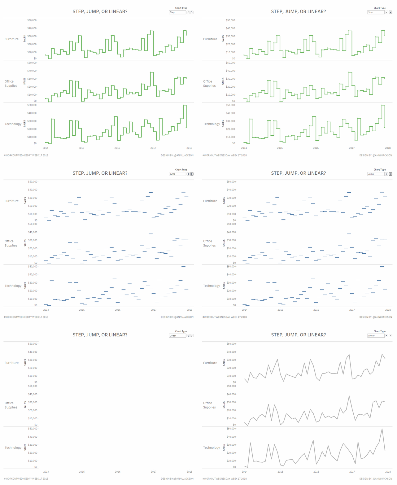
The workout this week is very straight forward – explore the different types of line charts (step lines, jump lines, and linear/normal lines). Don’t use the new built in features of 2018.1 (beta or release, depending on when you’re reading) found by clicking on the Path shelf. Instead use other functions or features to create the charts.

The tricky parts about this week’s workout will be the step lines. Pay special attention to the stop and start of the lines and where the tooltips display information. You are not allowed to duplicate the data or create a “path ID” field. Everything you do should be accomplished using a single connection of Superstore and no funny business.

Tiny additional element of creating the ability to flip through the chart types.

Requirements:
- Dashboard size 1000 x 800
- Displaying sales by month for each Category
- Create a button that flips through each chart type
- Match step line chart exactly, including tooltip, start/stop of lines, colors, labels
- Match jump line chart exactly, including axes, labels, tooltips
- Match normal line chart exactly, including axes, labels tooltips
This week uses the superstore dataset. You can get it here at data.world

After you finish your workout, share on Twitter using the hashtag #WorkoutWednesday and tag @AnnUJackson, @LukeStanke, and @RodyZakovich. (Tag @VizWizBI too – he would REALLY love to see your work!)

Also, don’t forget to track your progress using this Workout Wednesday form.
April 24, 2018
Workout Wednesday 14 | Guest Post | Frequency Matrix
Earlier in the month Luke Stanke asked if I would write a guest post and workout. As someone who completed all 52 workouts in 2017, the answer was obviously YES!

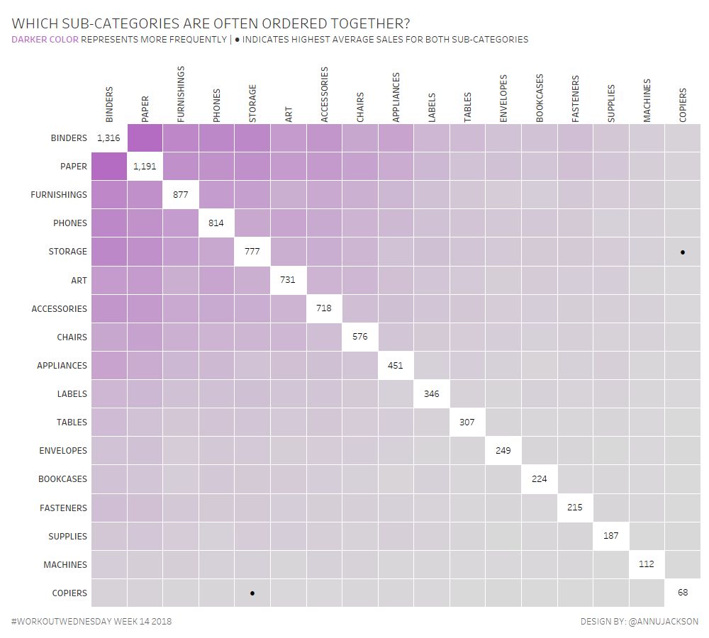
This week I thought I’d take heavy influence from a neat little chart made to accompany Makeover Monday (w36y2017) – the Frequency Matrix.

I call it a Frequency Matrix, you can call it what you will – the intention is this: use color to represent the frequency (intensity) of two things. So for this week you’ll be creating a Frequency Matrix showing the number of orders within pairs of sub-categories.

click to view on Tableau Public

Primary question of the visualization: Which sub-categories are often ordered together?
Secondary question of the visualization: How much on average is spent per order for the sub-categories.
Tertiary question: Which sub-category combination causes the most average spend per order?

Requirements
- Use sub-categories
- Dashboard size is 1000 x 900; tiled; 1 sheet
- Distinctly count the number of orders that have purchases from both sub-categories
- Sort the categories from highest to lowest frequency
- White out when the sub-category matches and include the number of orders
- Calculate the average sales per order for each sub-category
- Identify in the tooltip the highest average spend per sub-category (see Phones & Tables)
- If it’s the highest average spend for both sub-categories, identify with a dot in the square
- Match formatting & tooltips – special emphasis on tooltip verbiage
This week uses the superstore dataset. You can get it here at data.world

After you finish your workout, share on Twitter using the hashtag #WorkoutWednesday and tag @AnnUJackson, @LukeStanke, and @RodyZakovich. (Tag @VizWizBI too – he would REALLY love to see your work!)

Also, don’t forget to track your progress using this Workout Wednesday form.

Hints & Detail
- You may not want to use the WDC
- Purple is from hue circle
- You’ll be using both LODs and Table Calculations
- I won’t be offended if you change the order of the sub-category labels in the tooltips
- Dot is ●
- Have fun!
March 29, 2018