Tag: sentiment analysis
-
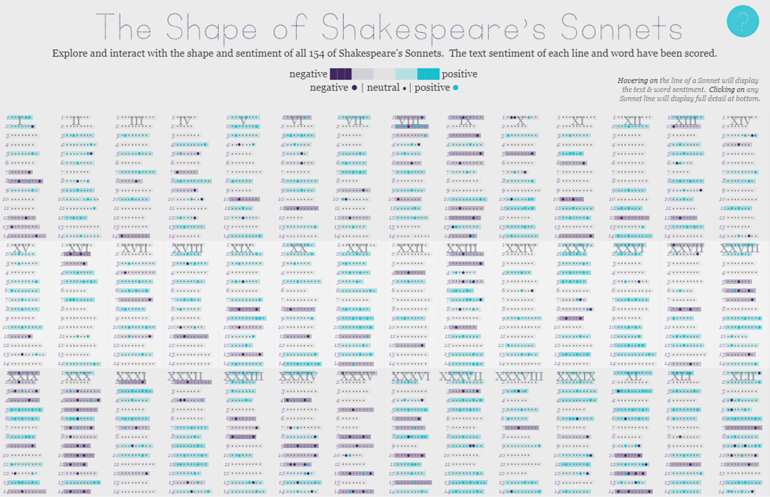
The Shape of Shakespeare’s Sonnets | #IronViz Books & Literature
Jump directly to the viz If it’s springtime that can only mean that it’s time to begin the feeder rounds for Tableau’s Iron Viz contest. The kick-off global theme for the first feeder is books & literature, a massive topic with lots of room for interpretation. So without further delay, I’m excited to share my…
-
And so it beings – Adventures in Python
Tableau 10.2 is on the horizon and with it comes several new features – one that is of particular interest to me is their new Python integration. Here’s the Beta program beauty shot: Essentially what this will mean is that more advanced programming languages aimed at doing more sophisticated analysis will become an easy to…